CSE 6242 / CX 4242: Homework 3 : Hadoop, Spark, AWS and Azure Solution

Description

Introduction

In this assignment you will be working with big data analytics using a variety of modern technologies. The dataset which you will be working on for the bulk of the assignment comes from the New York City Taxi & Limousine Commision (TLC). Further details on this dataset are available here. In Q1, you will be doing Java programming to become familiar with Hadoop and MapReduce. In Q2 you will perform further analysis with DataBricks, Scala and Spark, which are tools for working with large datasets. In Q3 you will perform large scale analysis in AWS using EMR and Pig. For Q4 you will work in Microsoft Azure and further hone your MapReduce abilities. Finally, in Q5 you will do some Machine Learning, utilizing Azure ML Studio.

A main goal of this assignment is to help students gain exposure to a variety of tools that they may use in future (e.g., future project, research, career). That is also why we intentionally include both AWS and Azure (most courses use only one), because we want students to be able to try and compare them (both platforms evolve rapidly), so in the future should they need to select a cloud platform to use, they can make more informed decisions and to be able to get started right away. You may find that a number of computational tasks in this assignment are not very difficult, and there seems to be quite a bit of “setup” to do before getting to the actual “programming” part of the problem. A main reason for this design is because for many students this assignment is the very first time they use any cloud services; they are new to the pay-per-use model, and they have never used a cluster of machines. There are over 1000 students in CSE 6242 (campus and online) and CX 4242 combined. This means we have students coming from a great variety of backgrounds. We wished we could provide every student unlimited AWS/Azure credit so that they can try out many services and write programs that are more complex. Over the past offering of this course, we have been gradually increasing the “programming” part and reducing much of the “setup” (e.g., the use of VM and Databricks notebook were major improvements). We will continue to further reduce the setup that students need to perform in future offerings of this course.

Q1 [15 points] Analyzing trips data with Hadoop/Java

Follow these Instructions to download, setup a preconfigured virtual machine (VM) image that you will use for this assignment.

Why use VMs? In earlier iterations of this course, students installed software on their own machines, and we (both students and instructor team) ran into all sorts of issues, some of which could not be resolved satisfactorily. The VM approach allows students to start working on the tasks much more quickly. We continue to experiment with other alternatives, so in the future, this may become even easier for our students!

Imagine that your boss gives you a large dataset which contains trip information of New York City Taxi and Limousine Commission (TLC). You are asked to provide the number of trips from each pickup point along with the total amount of fare. This information might help in positioning taxis depending on the demand at each location.

 

First, go over the Hadoop word count tutorial to familiarize yourself with Hadoop and some Java basics. You will be able to complete this question with only some knowledge about Java. Make sure you have already loaded the two trips data files into the HDFS file system in your VM (following the instructions mentioned in the beginning of this question). Each line in the file represents a trip’s information consisting of four columns:
PickUpLocationId, DropOffLocationId, Distance, Total Fare
separated by commas (,). Below is a small toy data example, for illustration purposes (on your screen, the text may appear out of alignment).

 

PickUpId, DropOffId, Distance,  TotalFare

1,        30,        20.2,      30.1

1,        24,        19.1,      28.2

2,        20,        18.3,      20.1

1,        31,        20.2,      33

1,        20,        0,         2.5

 

Your code should accept two arguments. The first argument (args[0]) will be a path for the input graph file on HDFS (e.g., data/trip1.csv), and the second argument (args[1]) will be a path for output directory on HDFS (e.g., data/q1output1). The default output mechanism of Hadoop will create multiple files on the output directory such as part-00000, part-00001, which will be merged and downloaded to a local directory by the supplied run script. Please use the run1.sh and run2.sh scripts for your convenience.

 

For each pickup location ID, compute the total number of trips that originate from that location and the total fare.

Requirements:

1. Output format: each line contains a PickupLocationID, followed by a tab (t), and then the expected “TotalNumberOfTrips,TotalAmount” tuple (without the quotes; and no space character before or after the comma)
2. Lines in output do not need to be sorted
3. Exclude trips that do not have pickup locations.
4. Exclude trips whose distance equals zero
5. Exclude trips whose total fare is less than or equal to zero
6. Your input must not have any column headers
7. Your output must not include column headers
8. In your output, round the total fare amount to two decimal points.

10.236 -> 10.24

10.235 -> 10.24

10.234 -> 10.23

10.2 -> 10.20

9. In your output TotalFares greater than 1,000 should contain thousands separators (a , for every 3 digits).

            1000.00 -> 1,000.00

            10100.00 -> 10,100.00

The following example result is computed based on the toy example above.

PickupId        TotalNoOfTrips,TotalFare 

1                     3,91.30

2                 1,20.10

We are not considering the <1, 20, 0, 2.5> record for computing the total number of trips and total fare for pick up location 1 because the distance was 0.

 

Deliverables

 

1. [5 points] Your Maven project directory including Q1.java. Please see the detailed submission guide at the end of this document. You must implement your own MapReduce procedure and must not import external graph processing libraries.

 

      2.         [5 points] q1output1.tsv: the output file of processing trip1.csv by run1.sh.

[5 points] q1output2.tsv: the output file of processing trip2.csv by run2.sh.

Q2 [25 pts] Analyzing a dataset with Spark/Scala on Databricks

Tutorial: First, go over this Spark on Databricks Tutorial, to get the basics of creating Spark jobs, loading data, and working with data.

You will analyze nyc-tripdata.csv^[1] using Spark and Scala on the Databricks platform. The dataset is a modified record of the NYC Green Taxi trips and includes information about the pick-up and drop-off dates/times, pick-up and drop-off locations, trip distances, fare amounts, payment types, and driver-reported passenger counts.

VERY IMPORTANT: Rename your notebook as q2-yourGTusername (e.g. q2-jdoe3) before submitting. Refer to the Databricks Setup Guide (open the link in a private browser window if you get ‘Permission Denied’ message) on how to rename the notebook.

Your objectives:

1. Filter the data to only keep the rows where the pickup location is different from the drop location and the trip distance is strictly greater than 2.0 (>2.0). Very important: all subsequent operations must be performed on this filtered dataframe.
2. List the top-5 most popular drop locations, sorted in descending order. If there is a tie, then the one with a lower location ID gets listed first.
3. List the top-5 most popular pickup locations, sorted in descending order. If there is a tie, then the one with a lower location ID gets listed first.
4. List the top-5 most popular pickup-dropoff pairs, sorted in descending order. If there is a tie, then one with a lower pickup location ID gets listed first.
5. List by days, the number of drop-offs over the period from January 1, 2019 (including January 1) to January 5, 2019 (including January 5). List the entries by day from January 1 to January 5.
6. List the top-3 locations with the maximum overall activity, i.e. sum of all pickups and all drop-offs at that location. In case of a tie, the lower location ID gets listed first.

You should perform this task using the DataFrame API in Spark. Here is a guide that will help you get started on working with data frames in Spark.

A template Scala notebook, q2.dbc has been included in the HW3-Skeleton that reads in a data file nyc-tripdata.csv. In the template, the input data is loaded into a dataframe, inferring the schema using reflection (Refer to the guide above).

Note: You must use only Scala DataFrame operations for this task. You will lose points if you use SQL queries, Python, or R to manipulate a dataframe.

Hint: You may find some of the following DataFrame operations helpful:

toDF, join, select, groupBy, orderBy, filter

Upload the data file nyc-tripdata.csv and q2.dbc to your Databricks workspace before continuing.  Follow the Databricks Setup Guide (open the link in a private browser window if you get ‘Permission Denied’ message) for further instructions.

List the results of the above task in the provided q2-results.csv file under the relevant sections. You must manually enter the output generated into the corresponding sections of the q2-results.csv file. (For generating the output in the Scala notebook, refer to show() and display()functions of Scala)

Deliverables

1. [10 pts]

1. q2-yourGTusername.dbc: Your solution as Scala Notebook archive file (.dbc) exported from Databricks. See the Databricks Setup Guide on creating an exportable archive for details.
2. q2-yourGTusername.scala: Your solution as a Scala source file exported from Databricks. See the Databricks Setup Guide on creating an exportable source file for details.
3. q2-yourGTusername.html: Your solution as a HTML file exported from Databricks. See the Databricks Setup Guide on how to export your code as an HTML.

Note: You should export your solution in all the three formats – .dbc, .scala and .html.

2. [15 pts] q2-results.csv: The output file of processing nyc-tripdata.csv from the q2 notebook file. You must copy the outputs of the display()/show() function into file titled q2-results.csv under the relevant sections.

Q3 [35 points] Analyzing Large Amount of Data with Pig on AWS

You will try out Apache Pig for processing data on Amazon Web Services (AWS). This is a fairly simple task, and in practice you may be able to tackle this using commodity computers (e.g., consumer-grade laptops or desktops). However, we would like you to use this exercise to learn and solve it using distributed computing on Amazon EC2, and gain experience (very helpful for your career), so you will be prepared to tackle problems that are more complex.

The services you will primarily be using are Amazon S3 storage, Amazon Elastic Cloud Computing (EC2) virtual servers in the cloud, and Amazon Elastic MapReduce (EMR) managed Hadoop framework.

For this question, you will only use up a very small fraction of your $100 credit.

AWS Guidelines

Please read the AWS Setup Tutorial provided to set up your AWS account. Instructions are provided both as a written guide, and a video tutorial.

Datasets

In this question, you will use a dataset of trips provided by the New York City Taxi and Limousine Commision (TLC). Further details on this dataset are available here and here. Using these links you can explore the structure of the data, however you will be accessing the dataset directly through AWS via the code outlined in the homework skeleton. You will be working with two samples of this data, one small, and one much larger.

VERY IMPORTANT: Both the datasets are in the US East (N. Virginia) region. Using machines in other regions for computation would incur data transfer charges. Hence, set your region to US East (N. Virginia) in the beginning (not Oregon, which is the default). This is extremely important, otherwise your code may not work and you may be charged extra.

Goal

You work at NYC TLC, and since the company bought a few new taxis, your boss has asked you to determine where good locations for the taxi drivers to frequent so as to pick up more passengers. Of course, the more profitable the locations are, the better. Your boss also tells you not to worry about short trips for any of your analysis, so only analyze trips which are 2 miles or longer.

You will be analyzing yellow taxi trips and green taxi trips together, i.e., perform your analysis on the “union” of those trips.

First, find the 20 most popular drop off locations in the Manhattan borough by finding which of these destinations had the greatest passenger count.

Now, analyze all pickup locations, regardless of borough. For each pickup location, determine the average total amount per trip and the proportion of trips starting at that pickup location that would end at one of the most popular drop off locations (i.e., proportion = number of trips that start at pick up location and end at a popular destination / total  number of trips that start at that pick up location). In other words, these two values represent the average amount of money TLC would make for a trip starting at that location and the probability it will end up at one of the most popular destinations. Multiply the average total amount value and the proportion value, to weigh the income  made based on the probability of passengers going to the popular destinations.

Bear in mind, your boss is not as savvy with the data as you are, and is not interested in location IDs. To make it very easy for your boss, provide the Borough and Zone for each of the top 20 pick up locations you determined. To help you evaluate the correctness of your output, we have provided you with the output for the small dataset.

Note: Please strictly follow the formatting requirements for your output as shown in the small dataset output file. You can use https://www.diffchecker.com/ to make sure the formatting is correct. Improperly formatted outputs may not receive any points, as we may not know how to interpret them.

Loading data in PIG

You are provided with two Pig files in the skeleton. One defines the small data set, and the other defines the large one. Go through them to find out which fields are available and how they are typed. Do not change any of the code already provided in the files

Data will be loaded into 3 relations (a construct in Pig similar to variables).

1. green (Data from Green Taxi trips)
2. yellow (Data from Yellow Taxi trips)
3. locations (Relates to the PULocationID and DOLocationID in green and yellow)

Using PIG (Read these instructions carefully)

There are two methods to debug PIG on AWS (all instructions are in the AWS Setup Tutorial):

1. Use the interactive PIG shell provided by EMR to perform this task from the command line (grunt). Refer to Section 5 in the AWS Setup Tutorial for a detailed step-by-step procedure. You should use this method if you are using PIG for the first time as it is easier to debug your code. However, as this method requires  a persistent ssh connection to your cluster until your task is complete, it is suitable only for the smaller dataset.

2. Upload a PIG script with all the commands which computes and direct the output from the command line into a separate file. Once you verify the output on the smaller dataset, use this method for the larger dataset. You do not have to ssh or stay logged into your account. You can start your EMR job, and come back after the job is complete! This is covered in Section 6 of the tutorial.

Note: In summary, verify the output for the smaller dataset with Method 1 and submit the results for the bigger dataset using Method 2.

Note:

• Refer to other commands such as LOAD, USING PigStorage, FILTER, GROUP, ORDER BY, FOREACH, GENERATE, LIMIT, STORE, UNION, JOIN, etc.

• Your script will fail if your output directory already exists. For instance, if you run a job with the output folder as s3://cse6242-<GT account username>/output-small, the next job which you run with the same output folder will fail. Hence, please use a different folder for the output for every run.

Deliverables

1. [15 pts] pig-script.txt: The PIG script for the question (using the larger data set).

2. [20 pts] pig-output.txt: Output (tab-separated) (using the larger data set).

Note: Please strictly follow the guidelines below, otherwise your answer may not be graded.

1. Ensure that file names (case sensitive) are correct.
2. Ensure file extensions (.txt) are correct.
3. Double check that you are submitting the correct set of files — we only want the script and output from the larger dataset. Also double check that you are writing the right dataset’s output to the right file.
4. You are welcome to store your script’s output in any bucket you choose, as long as you can download and submit the correct files.
5. Do not make any manual changes to the output files

Q4 [35 points] Analyzing a Large Datasets using Hadoop on Microsoft Azure

VERY IMPORTANT: Use Firefox or Chrome in incognito/private browsing mode when configuring anything related to Azure (e.g., when using Azure portal), to prevent issues due to browser caches. Safari sometimes loses connections.

Goal

The goal of this question is to familiarize you with creating cluster/storage and running MapReduce programs on Microsoft Azure. Your task is to write two separate MapReduce programs for NYC Taxi & Limousine Commission Dataset to compute (a) compute the distribution of degree differences of locations; (b) the average fare for different passenger counts (see example below). Note that this question shares some similarities with Question 1 (e.g., both are analyzing graphs). Question 1 can be completed using your own computer. This question is to be completed using Azure. We recommend that you first complete Question 1. Please carefully read the following instructions.

You will use the data file data.tsv^[2] (~ 7.6 million rows). Each line represents a single taxi trip consisting of four tab-separated values: PickUpLocationID, DropOffLocationID, PassengerCount, TotalFare.

PickUpLocationID and DropOffLocationID are positive integers. We view this dataset as a graph (or network) of locations, where each node in this graph is a location ID (PickUpLocationID or DropOffLocationID) and we connect two location IDs with a separate directed edge for each trip that goes from the “Source” location (PickUpLocationID) to the “Target” location (DropOffLocationID). Every trip is shown as a separate directed edge.

PickUpLocationID	DropOffLocationID	PassengerCount	TotalFare
264	264	5	4.3
97	49	2	7.3
49	189	2	5.8
189	17	2	19.71
264	264	1	19.3
49	17	1	7.8

Your code should accept two arguments upon running. The first argument (args[0]) will be a path for the input graph file, and the second argument (args[1]) will be a path for output directory. The default output mechanism of Hadoop will create multiple files on the output directory such as part-00000, part-00001, which will have to be merged and downloaded to a local directory (instructions on how to do this are provided below).

4a. Compute distribution of degree differences for locations

Each line of your output is of the format:

diff        count

1. diff is a node’s out-degree minus its in-degree
2. count is the number of nodes that have the value of diff (specified in 1)
3. Separate diff and count by a tab (t) character
4. Lines in your output do not need to be sorted
5. Do not add any header or column name to your output
6. All values in the output should be integer

The out-degree of a node (location ID) is the number of edges where that node is the Source (PickUpLocationID). The in-degree of a node is the number of edges where that node is the Target (DropOffLocationID). When the source and target are the same node, that self-loop contributes to both the node’s in-degree and out-degree. For example, in the above table, there are two entries of 264→264, then both in-degree and out-degree of node 264 will be 2.

The following result is computed based on the data above.

-2        1

0        2

1        2

Output	Explanation
-2        1	There is 1 node (node 17) whose degree difference is -2
0        2	There are 2 nodes (node 264,node 189) whose degree difference is 0.
1        2	There are 2 nodes (node 49,node 97) whose degree difference is 1.

Hint​: One way of accomplishing this task is to use the mapreduce procedure twice. The first one for finding the difference between out-degree and in-degree for each node, the second for calculating the node count of each degree difference. You will need to make changes in the skeleton code for this.

4b. Compute average fare for different passenger counts

Each line of your output is of the format:

PassengerCount        AverageFare

1. PassengerCount is the set of the third column of the data
2. AverageFare is the average fare for different PassengerCount
3. Separate PassengerCount and AverageFare by a tab (t) character 
4. Lines in your output do not need to be sorted
5. Do not add any header or column name to your output
6. The PassengerCount in the output should be integer
7. The AverageFare must be rounded to 2 decimal places

The following result is computed based on the data above.

1        13.55

2        10.94

5        4.30

Output	Explanation
1        13.55	There are 2 rows for PassengerCount=1 The average fare (19.3 + 7.8) / 2 = 13.55
2        10.94	There are 3 rows for PassengerCount=2 The average fare is (7.3 + 5.8 + 19.71) / 3 = 10.94
5        4.30	There is 1 row for PassengerCount=5 The average fare is 4.30

In the Q4 folder of the hw3-skeleton, you will find the following files we have prepared for you in a and b subfolders:

• src directory contains a main Java file that you will work on. We have provided some code to help you get started. Feel free to edit it and add your files in the directory, but the main class must be called “Q4a” and “Q4b”.
• pom.xml contains necessary dependencies and compile configurations for the question.

To compile, you can run the command in the directory which contains pom.xml.

mvn clean package

This command will generate a single JAR file in the target directory (i.e., a/target/q4a-1.0.jar or b/target/q4b-1.0.jar).

Creating Clusters in HDInsight using the Azure portal

Azure HDInsight is an Apache Hadoop distribution. This means that it handles large amounts of data on demand. The next step is to use Azure’s web-based management tool to create a Linux cluster. Follow the recommended steps shown here (or the full Azure’s documentation here) to create a new cluster.

At the end of this process, you will have created and provisioned a New HDInsight Cluster and Storage (the provisioning will take some time depending on how many nodes you chose to create). Record the following important information (we also recommend that you take screenshots) so you can refer to them later:

• Cluster login credentials
• SSH credentials
• Resource group
• Storage account
• Container credentials

VERY IMPORTANT: HDInsight cluster billing starts once a cluster is created and stops when the cluster is deleted. Thus, you should delete your cluster when it is no longer in use. You can find all clusters and storages you have created in “All resources” on the left panel.  Please refer to the official Azure documentation here for how to delete an HDInsight cluster.

Uploading data files to HDFS-compatible Azure Blob storage

We have listed the main steps from the documentation for uploading data files to your Azure Blob storage here:

1. Follow the documentation here to install Azure CLI.
2. Open a command prompt, bash, or other shell, and use az login command to authenticate to your Azure subscription. When prompted, enter the username and password for your subscription.
3. az storage account list command will list the storage accounts for your subscription.
4. az storage account keys list –account-name <storage-account-name> –resource-group <resource-group-name> command should return “key1” and “key2”. Copy the value of “key1” because it will be used in the next steps.
5. az storage container list –account-name <storage-account-name> –account-key <key1-value> command will list your blob containers.
6. az storage blob upload –account-name <storage-account-name> –account-key <key1-value> –file <data.tsv> –container-name <container-name> –name <new-blob-name>/<data.tsv> command will upload the source file to your blob storage container. <new-blob-name> is the folder name you will create and where you would like to upload tsv files to. If the file is uploaded successfully, you should see “Finished [#####] 100.0000%”.

Using these steps, upload data.tsv to your blob storage container. The uploading process may take some time. After that, you can find the uploaded files in storage blobs at Azure (portal.azure.com) by clicking on “Storage accounts” in the left side menu and navigating through your storage account
(<”All resources” in the panel> → <Your Storage Account> → <Select your container to which you’ve uploaded the dataset> → <Select the relevant blob folder>).
For example, “jonDoeStorage” → “jondoecontainer-xxx” → “jdoeData” → “data.tsv”.
After that write your hadoop code locally and convert it to a jar file using the steps mentioned above.

Uploading your Jar file to HDFS-compatible Azure Blob storage

Azure Blob storage is a general-purpose storage solution that integrates with HDInsight. Your Hadoop code should directly access files on the Azure Blob storage.

Upload the jar file created in the first step to Azure storage using the following command (here we take q4a-1.0.jar as an example, and you need to repeat steps for q4b-1.0.jar):

scp <your-relative-path>/q4a-1.0.jar <ssh-username>@<cluster-name>-ssh.azurehdinsight.net:

You will be asked to agree to connect by typing “yes” and your cluster login password. Then you will see q4a-1.0.jar is uploaded 100%.

SSH into the HDInsight cluster using the following command:

ssh <ssh-username>@<cluster-name>-ssh.azurehdinsight.net

<ssh-username> is what you have created in step 10 in the flow.

Note: if you see the warning – REMOTE HOST IDENTIFICATION HAS CHANGED, you may clean /home/<user>/.ssh/known_hosts” by using the command rm ~/.ssh/known_hosts. Please refer to host identification.

 

Run the ls command to make sure that the q4a-1.0.jar file is present.

To run your code on the data.tsv file, run the following command:

yarn jar q4a-1.0.jar edu.gatech.cse6242.Q4a wasbs://<container-name>@<storage-account-name>.blob.core.windows.net/<new-blob-name>/data.tsv wasbs://<container-name>@<storage-account-name>.blob.core.windows.net/degreeoutput

Command format: yarn jar jarFile packageName.ClassName dataFileLocation outputDirLocation

Note: if “Exception in thread “main” org.apache.hadoop.mapred.FileAlreadyExistsException…” occurs, you need to delete the output folder and files from your Storage. You can do this at portal.azure.com. Click “All resources” in the left panel, you will see you storage and cluster. Click your storage, then your container, you will see all folders created by you and the “degreeoutput” folder. You need to click “Load more” at the bottom to see all folders/files. You need to delete output at different places: 1. degreeoutput; 2. user/sshuser/*

The output will be located in the directory: wasbs://<container-name>@<storage-account-name>.blob.core.windows.net/degreeoutput

If there are multiple output files, merge the files in this directory using the following command (you may see there is only one output file and no need to merge, but there is no hurt to run this command):

hdfs dfs -cat wasbs://<container-name>@<storage-account-name>.blob.core.windows.net/degreeoutput/* > degree.out

Command format: hdfs dfs -cat location/* >outputFile

Then you may exit to your local machine using the command:

exit

You can download the merged file to the local machine (this can be done either from Azure Portal or by using the scp command from the local machine). Here is the scp command for downloading this output file to your local machine:

scp <ssh-username>@<cluster-name>-ssh.azurehdinsight.net:/home/<ssh-username>/degree.out <your local directory>

Using the above command from your local machine will download the degree.out file into the local directory. Repeat this process to download average.out. Make sure your output file has exactly two columns of values as shown above. Your output files should be able to be opened and readable in text editors like notepad++. The extension MUST be exactly “.out”, NOT “.txt.out”, “.tsv.out” or others. You should implement your own map/reduce procedure and should not import external graph processing library.

Deliverables

1. [8pt] Q4a.java & q4a-1.0.jar: Your java code and converted jar file for Q4a.

2. [7pt] Q4b.java & q4b-1.0.jar: Your java code and converted jar file for Q4b.

3. [10pt] degree.out: the output file generated after processing data.tsv.

4. [10pt] average.out: the output file generated after processing data.tsv.

Q5 [10 points]  Regression: Automobile price prediction, using Azure ML Studio

Note: Create and use a free workspace instance on Azure Studio instead of your Azure credit for this question. Please use your Georgia Tech username (e.g., jdoe3) to login.  

Goal

The main purpose of this question is to introduce you to Microsoft Azure Machine Learning Studio and familiarize you with its basic functionality and typical machine learning workflow. Go through the “Automobile price prediction” tutorial and complete the tasks below.

You will modify the given file, results.csv, by adding your results for each of the tasks below. We will autograde your solution, therefore DO NOT change the order of the questions.  Report the exact numbers that you get in your output, and DO NOT round any numbers.

1. Update your GT username in the results.csv file to replace gburdell3.
2. [3 points] Repeat the experiment mentioned in the tutorial and report the values of the metrics as mentioned in the ‘Evaluate Model’ section of the tutorial.
3. [3 points] Repeat the same experiment, change the ‘Fraction of rows in the first output’ value in the split module to 0.8 (originally set to 0.75) and report the corresponding values of the metrics.
4. [4 points] Evaluate the model with the 5-fold cross-validation (CV), select the parameters in the module ‘Partition and sample’ (Partition and Sample) (see figure below). Report the values of Root Mean Squared Error (RMSE) and Coefficient of Determination for each fold. (1st fold corresponds to fold number 0 and so on).

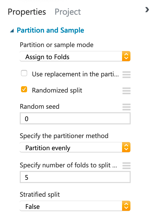
Figure: Property Tab of Partition and Sample Module

To summarize, in order to complete sub question 4, you need to do the following:

1. Import the entire dataset (Automobile Price Data (Raw))
2. Clean the missing data by removing rows that have any missing values
3. Partition and Sample the data.
4. Create a new model (Linear Regression)
5. Finally, perform cross validation on the dataset.
6. Visualize/Report the values.

Deliverables

1. [10pt] results.csv: a csv file containing results for all of the three parts.

Important: folder structure of the zip file that you submit

You are submitting a single zip file HW3-GTUsername.zip (e.g., HW3-jdoe3.zip, where “jdoe3” is your GT username), which must unzip to the following directory structure (i.e., a folder “HW3-jdoe3”, containing folders “Q1”, “Q2”, etc.). The files to be included in each question’s folder have been clearly specified at the end of each question’s problem description above.

HW3-GTUsername/      

    Q1/

        src/main/java/edu/gatech/cse6242/Q1.java

        pom.xml

        run1.sh

        run2.sh

        q1output1.tsv

        q1output2.tsv

        (do not attach target directory)

    Q2/

        q2-yourGTusername.dbc

        q2-yourGTusername.scala

        q2-yourGTusername.html

        q2-results.csv

    Q3/

        pig-script.txt

        pig-output.txt

    Q4/

        a/

src/main/java/edu/gatech/cse6242/Q4a.java

pom.xml

        b/

src/main/java/edu/gatech/cse6242/Q4b.java

                  pom.xml

          q4a-1.0.jar (from target directory)

  q4b-1.0.jar (from target directory)

          degree.out

          average.out

       (do not attach target directory)

    Q5/

        results.csv